

Putting a 1×8 splitter into a budget as 9 dB, or a 1×16 as 12 dB, is the fastest way to build a PON that tests short on the first power-meter reading. The 10 × log10(N) figure is only the ideal share of light each port can receive. The number that belongs in the spreadsheet is the maximum insertion loss, measured with connectors fitted, at the test wavelengths the vendor actually used. For our 1×N series that is 10.5 dB at eight ports and 13.8 dB at sixteen, both at λ = 1310/1550 nm with connectors included.
The gap between those two ideas is not slack in a well-made part. It is the excess loss of the chip, the fibre-to-chip coupling, the packaging, and the two connector interfaces the light crosses on its way in and out. The Fiber Optic Association's splitter testing reference states this directly: what a standard double-ended test measures is the loss due to the split ratio, the excess loss from manufacturing, and the input and output connectors together. A designer who budgets the split ratio alone leaves every one of those terms to be discovered in the field.
Ideal splitting loss versus maximum insertion loss
Equal splitting of one input into N outputs divides the power evenly, so each port receives 1/N of it. In decibels that is:
Ideal splitting loss (dB) = 10 × log10(N)
For 1×4 that is 6.02 dB, for 1×8 it is 9.03 dB, for 1×16 it is 12.04 dB, for 1×32 it is 15.05 dB, and for 1×64 it is 18.06 dB. Each doubling of the port count adds 3.01 dB, which is why the split-ratio ladder reads as a sequence of three-decibel steps above the first split.
Insertion loss is that ideal figure plus everything the device adds. Because a splitter is passive, no gain can offset the extra loss somewhere downstream; every tenth of a decibel the part contributes reduces the optical power at the receiver, and that reduction happens before any fibre, splice or patch-cord loss is counted.
The distinction bites hardest at the top of the ratio range, where the excess term grows faster than the ideal term. Between our 1×4 and 1×8 the maximum insertion loss rises from 7.4 to 10.5 dB, close to the ideal 3.01 dB of the doubling. Between 1×8 and 1×16 it rises 3.3 dB, and between 1×32 and 1×64 it rises 3.3 dB again. A designer who scales from the ideal ladder therefore understates the 16-way stage by about half a decibel more than the 8-way stage, and the 64-way stage by about a decibel more. Small numbers, but they land at the end of a budget that already carries connector, splice and margin terms.
1×N and 2×N maximum insertion loss by split ratio
The table below is the maximum insertion loss from our splitter parameter tables. Every value applies to a device with all integrated components and connectors included, tested at λ = 1310/1550 nm, over a 1260–1650 nm operating band. The same figures appear on the subrack, plug-in, tray, box and miniature steel-tube series pages, so the budget does not change with packaging.
| Split ratio | Ideal splitting loss (dB) | 1×N max insertion loss (dB) | 2×N max insertion loss (dB) | Overhead over ideal, 1×N (dB) |
|---|---|---|---|---|
| 1×4 / 2×4 | 6.02 | 7.4 | 7.7 | 1.38 |
| 1×8 / 2×8 | 9.03 | 10.5 | 10.8 | 1.47 |
| 1×16 / 2×16 | 12.04 | 13.8 | 14.1 | 1.76 |
| 1×32 / 2×32 | 15.05 | 17.1 | 17.4 | 2.05 |
| 1×64 / 2×64 | 18.06 | 20.4 | 20.6 | 2.34 |
The 2×N column is a separate product family, not a restatement of the 1×N figures. Two-input devices carry a slightly higher maximum loss at every ratio, 7.7 dB at 2×4 rising to 20.6 dB at 2×64. Substituting one column for the other in a spreadsheet is a common error when a project moves to a protected or dual-feeder layout, and it understates the stage by only 0.2–0.3 dB at the ratios shown here — enough to matter when the 2×N part is the one actually installed.
Read the last column as a tolerance allowance rather than a property of the split. It is the difference between the worst device our tables permit and the physics of dividing light, and it widens with port count because more waveguide branches mean more chances to accumulate loss. A 1×64 stage at 20.4 dB already spends 2.34 dB above its ideal share before a single fibre metre is added.
What the test conditions do to your number
Three conditions in those tables are easy to miss when a datasheet is copied into a bill of materials, and each of them changes the value you should carry.
The first is "connectors included". Our table values already contain the loss of the input and output connector interfaces, so the splitter line in a budget should not be split again into a device loss plus a separate patch-cord allowance at the splitter ports. If a vendor quotes a device-only figure, the interface loss has to be added back before the two tables can be compared.
The second is the test wavelength, λ = 1310/1550 nm. Those are the wavelengths at which the maximum insertion loss numbers were taken. They cover the dominant downstream and upstream windows of a typical PON deployment, but they are not a statement about the part at 1490 nm or at 1625 nm. The operating band of 1260–1650 nm says the device is intended to work across the full window; which wavelength your link budget must be computed at is set by the optics and the service mix, not by the splitter table.
The third is how the ports compare with each other. Our maximum splitting uniformity is 0.7 dB at four ports, 0.8 dB at eight, 1.0 dB at sixteen, 1.5 dB at thirty-two and 2.0 dB at sixty-four. Uniformity is the permitted spread between the best and worst output port; it is a different property from insertion loss and is not added to the maximum figure on the same line.
Uniformity, and the 0.5 dB band-edge adder
Uniformity is measured at 1310 nm, 1490 nm and 1550 nm. For the wavelength ranges 1260–1300 nm and 1600–1650 nm, the permitted uniformity value increases by 0.5 dB over the figure in the table. With a 1×16 stage, the worst port can therefore be 1.0 dB below the best port inside the three measured windows, and 1.5 dB below it in the band-edge ranges.
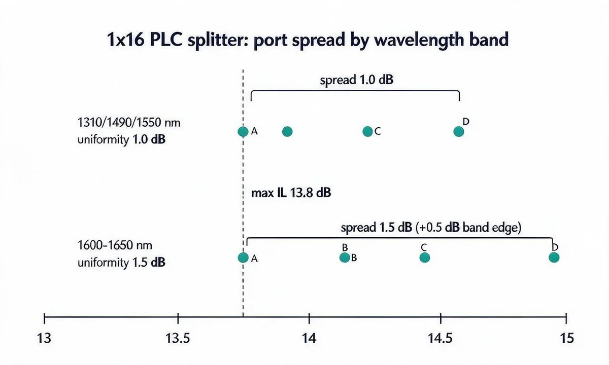
Where this changes a design decision is at the ends of the band. A link that uses a wavelength inside 1260–1300 nm or 1600–1650 nm can encounter a port 0.5 dB worse than the datasheet uniformity suggests, while a link that stays within the measured windows cannot exceed the tabulated spread. When comparing ports, or when a measured result sits close to the limit at a band-edge wavelength, use the tabulated uniformity plus 0.5 dB. At 1310, 1490 or 1550 nm, the tabulated spread is the figure to use.
Building the loss budget around the splitter
The splitter is one line among several, and treating it as the whole budget is the other common error. The Fiber Optic Association's loss budget guide defines the loss budget as the estimated average losses of every component in the cable plant added end to end, and states that the cable plant budget must consider transceiver wavelength, fibre type and link length plus the losses in splices, connections and other passive devices such as PON splitters. It also separates this from the power budget, which is the range between transmitter output and receiver sensitivity that the cable plant must fit inside.
For a singlemode access span, the passive terms are:
- Fibre attenuation over the route length at the wavelength being computed.
- Mated connections — every connector pair the light crosses, counted where it is mated rather than where a connector is attached.
- Fusion splices at closures and at pigtail joins.
- The splitter stage, at maximum insertion loss, once per stage.
The FOA quotes typical singlemode figures of 0.4 dB/km at 1310 nm and 0.3 dB/km at 1550 nm, factory-made singlemode connectors at 0.1–0.2 dB, and fusion splices typically under 0.05 dB, alongside TIA-568 allowances of 0.75 dB per connection and 0.3 dB per splice. Treat those as inputs for a design estimate, not as a substitute for the connectors and cable actually specified. Field-terminated singlemode connectors, which the FOA describes at 0.5–1.0 dB, are the usual reason a link sized on factory values comes up short.
Margin, and the reason not to use best-case values
The same guide recommends being conservative rather than designing on best-possible specifications, and points to a recommended excess margin for system degradation of as much as 3 dB, with a general rule that link loss margin should exceed about 3 dB. Sources age, connectors get mated, dirty or damaged, and a cut cable needs a repair splice; all of that consumes margin that does not exist if the budget was written at typical values.
Its treatment of measurement uncertainty is equally relevant after installation. A calculated budget assumes values for component losses and does not include the uncertainty of the measurement, so pass/fail judgement on a link measured within ±0.2–0.5 dB of the estimate needs care on both sides.
A worked budget you can reproduce
The arithmetic below is a planning example, not a product capability. It uses the values above and states each assumption so a different route can be recomputed with the same structure.
| Loss element | Assumption | Quantity | Loss (dB) |
|---|---|---|---|
| Feeder and distribution fibre at 1310 nm | 0.4 dB/km, FOA typical singlemode | 8 km | 3.20 |
| Mated connections | 0.2 dB per connection, FOA typical factory-made | 4 | 0.80 |
| Fusion splices | 0.05 dB each, FOA typical singlemode | 6 | 0.30 |
| 1×16 PLC splitter | Maximum insertion loss, connectors included, already stated for the output port | 1 | 13.80 |
| Excess margin | FOA general rule, above 3 dB | 1 | 3.00 |
| Total to clear | 21.10 |
The splitter line is deliberately the maximum value and nothing more. That figure is a maximum output-port insertion loss, so it already describes the worst output port; adding the 1.0 dB uniformity on top would charge the same penalty twice. Uniformity keeps its own job, which is to answer how far apart good and bad ports can be, not to raise the single worst-case number.
Read the 21.10 as the loss the link has to be able to tolerate, and compare it with the power budget of the optics you intend to use. The splitter accounts for 13.80 dB of that total, slightly under two-thirds of the number. Swapping the 1×16 for a 1×8 in the same route drops the splitter line to 10.5 dB and takes 3.3 dB out of the total, easing the optics needed for the span.
The method also works in reverse, which is where the excess-over-ideal column earns its place. When a proposed split ratio sits close to the limit of the available optics, the gap between the ideal and the maximum value for that stage is a fixed allowance to add before the margin conversation starts: 1.47 dB at 1×8, 1.76 dB at 1×16, 2.34 dB at 1×64. Those figures do not shrink because a link is short; they are part of the component.
What the 3 dB step between 1×8 and 1×16 actually costs
Every step up the ratio ladder subtracts about 3 dB from the share each subscriber receives, which halves the optical power arriving at each port. Halving the power is not a licence to halve the distance: reach is set at system level by the optics in use, their power budget, the remaining passive loss, and what the fibre and dispersion allow at the service's bit rate. Our splitter tables say nothing about distance, and the figures here should not be used to infer a maximum reach.
What the step does do is consume a specific quantity of the remaining budget. Against our maximum insertion losses, moving from 1×8 to 1×16 takes 3.3 dB out of what is left for fibre, connectors, splices and margin; going from 1×16 to 1×32 takes a further 3.3 dB. Compared with the rest of the passive path, the split ratio is the dominant lever: in the example above, fibre over 8 km costs 3.2 dB, so one step in split ratio consumes more budget than the entire 8 km route.
That is why split ratio is usually the last decision in a PON design, taken after the route, the connector and splice count and the optics class are known. When the ratio sits at the edge of what those optics tolerate, that 3.3 dB is the difference a 1×16 design lives without and a 1×8 design keeps, before any field degradation.
Centralized splitting versus cascaded splitting
Whether to split once in the central office, head-end cabinet or street cabinet, or to split in two stages, turns on where the splitters can be housed, how subscribers are distributed, and how much passive loss the budget can carry. Both arrangements produce the same number of ports from one optical line terminal port; they differ in where light is divided and how many interfaces it crosses.
The arithmetic of a two-stage split
Take a 32-way service area. A single 1×32 stage carries a maximum of 17.1 dB from our table. Building the same 32 ways from a 1×4 followed by 1×8 stages carries 7.4 + 10.5 = 17.9 dB of splitter maximum insertion loss, taking both values as published with their connectors included. On that like-for-like basis the two stages cost 0.8 dB more than one 1×32. That is the whole answer only if nothing else changes.
What the cascade adds on top depends on how the two stages are joined, and the published values cannot settle that for you. They are tested with connectors included, but how a 1×4 pigtail and a 1×8 pigtail are brought together in a given cascade decides which of those interfaces actually survive. If the joint is a mated connector pair the two tables do not already cover, the budget has to carry it: 0.2 dB at the FOA typical for a factory-made singlemode connection, closer to 0.5 dB if it is carried at field-terminated values. If the joint is a fusion splice inside a closure, splice loss, typically under 0.05 dB, is the addition. Where the build removes or replaces pigtail connectors that the tables assume are present, the published values no longer describe those ports, and the specification or test report for that build has to govern the splitter lines instead.
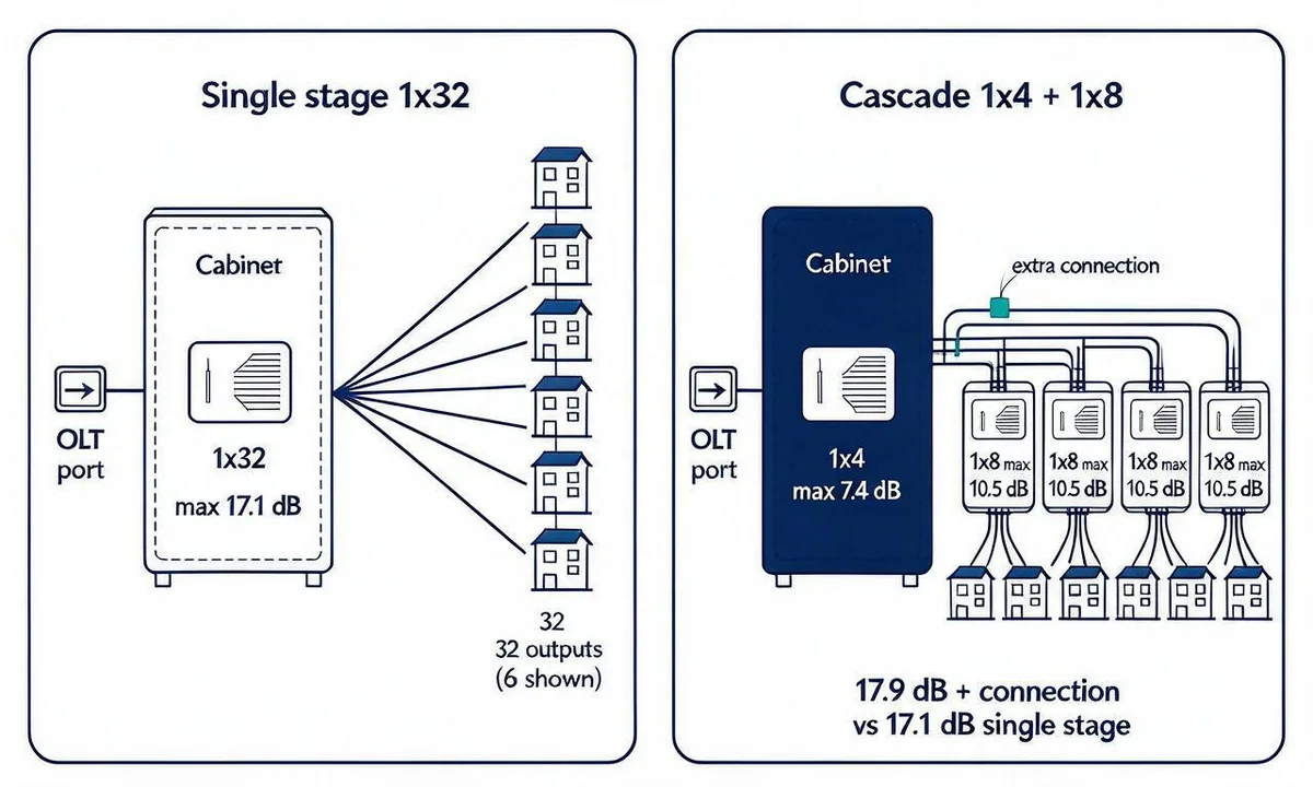
The cascade costs loss but buys placement. With a single stage, every subscriber is served from the point where the split happens, so its position must suit the whole service area. With two stages, the first split can sit in a cabinet that concentrates feeder traffic, and the second stages can be distributed into buildings or street cabinets closer to subscribers, each with its own 1×8 and its own housing.
When each arrangement earns its position
The lists below are conditions to test a proposed design against, not a ranking. Most of them are questions about the physical ODN rather than about light, and a design that answers several of them in one direction will usually lean that way.
A centralized single-stage split fits when:
- Subscribers in the service area are reasonably concentrated and all reachable from one cabinet, so no second split point is needed;
- The available optics carry the single-stage maximum insertion loss plus the route, connector and splice terms with margin left (17.1 dB at 1×32, 20.4 dB at 1×64);
- There is rack or cabinet space for the splitter module and the output pigtails at the single point where the split happens;
- Administration is simpler with one splitter record per PON port, or the operator's provisioning process expects it.
A two-stage cascade fits when:
- Subscribers are spread across several buildings or blocks far enough apart that a common serving point does not exist;
- The first split can be sized so that the second stage is filled by subscribers who actually exist, rather than by reserved capacity;
- The budget can carry the extra stage and its joint: 0.8 dB of published splitter loss against a single 1×32, plus the joint as built (splice or mated connection), plus the additional margin the design policy requires;
- New buildings or phases can be added by installing another second-stage splitter, without re-cabling the feeder.
Cascades turn sour in the other direction when the second stage is a large module placed to serve subscribers who arrive years later. The loss of that stage is incurred as soon as the feeder is lit, and the ports that sit unused carry no traffic while still having set the budget. A cascade sized to real demand and reloaded as demand grows keeps the trade honest; a cascade sized to maximum capacity trades loss and margin for flexibility nobody is using yet.
The physical form follows the same reasoning. Our splitter ranges include rack-mounted subrack units and plug-in modules for cross-connect cabinets, tray and box types for distribution frames and enclosures, and miniature steel-tube units that can be re-packaged into those housings. Choosing packaging that matches the chosen split point keeps interfaces where they are designed to be, instead of adding a patch-cord connection to move light between incompatible housings.
Procurement and acceptance checklist
Most disputes about splitter loss are settled before an order is placed, by reading three lines of a datasheet and one test report. Run through the following when comparing offers, and again when the goods arrive.
- Does the quoted maximum insertion loss state whether connectors are included? If a supplier quotes a device-only value, ask for the value with connectors fitted, because that is what the installed link sees.
- Which wavelengths were the insertion-loss values taken at? Verify that they match the wavelengths your budget is computed at, and ask what the part does at any other wavelength in the service mix.
- Is splitting uniformity stated with its test wavelengths and the edge-band adder? A uniformity figure without those conditions cannot be compared with another supplier's.
- Is the operating band stated, and does it cover every wavelength the service plan uses?
- Are the 1×N and 2×N tables separate? Ask for the correct column for the part being purchased, not a general split-ratio table.
- Is the connector grade specified? Our tables give minimum return loss of 45 dB (PC), 50 dB (UPC) and 55 dB (APC); a budget that assumes APC interfaces while the order ships PC will be short on reflectance even if insertion loss looks right.
- Is polarization-dependent loss within the value needed? Our tables permit 0.2 dB at 4 and 8 outputs and 0.3 dB at 16, 32 and 64 outputs.
- How will each port be tested, and against which 0 dB reference? The FOA reference allows the double-ended loss method with connectors on both ends or a single-ended method, and its worked example sets the source reference through a launch cable before reading each output through a receive reference cable. Either way, the report should name the reference method and state whether the result includes the device's connectors, so it can be compared with the maximum table.
When a result sits near the limit, remember that the measurement itself carries uncertainty, which the FOA puts at roughly ±0.2–0.5 dB for insertion-loss testing. A port measured 0.3 dB above the table value on a meter with that uncertainty is a conversation about the test setup before it is a rejected device.
Frequently asked questions
Should I use 9 dB or 10.5 dB for a 1×8 splitter?
Use 10.5 dB if you are budgeting our 1×N 1×8 with connectors, at 1310/1550 nm. The 9.03 dB figure is the ideal split alone and leaves out the excess loss and connector interfaces. If you are checking port-to-port spread rather than one worst-case number, the 0.8 dB uniformity at eight outputs is the figure for that question.
Can I use the same table for 2×N splitters?
No. Two-input devices have their own values, 7.7 dB at 2×4 through 20.6 dB at 2×64, and they are not the same numbers as the 1×N column. Take the column that matches the part on the order.
Does the 0.5 dB band-edge adder go into the insertion loss line?
It applies to uniformity, for wavelengths in 1260–1300 nm and 1600–1650 nm. Our tables do not specify a band-edge increase for maximum insertion loss, so the adder belongs to the port-spread question rather than to the 13.8 dB or 10.5 dB line.
Is a cascaded split always worse than a single stage?
On the published values alone, a 1×4 plus 1×8 cascade carries 17.9 dB against 17.1 dB for one 1×32, so 0.8 dB before any joint is counted. Add the joint as the build actually makes it: a mated pair about 0.2 dB at factory-made values and about 0.5 dB field-terminated, a fusion splice typically under 0.05 dB. If the build changes the connector and pigtail arrangement the table values were tested in, take the splitter loss from that build's specification or test result. The cascade is the better choice when subscribers are physically distributed and the first stage can be sized to real demand.
Does a lower split ratio guarantee a longer link?
No. Reach follows from the optics' power budget and the whole passive path, including route length, connections, splices and margin. A split-ratio table only tells you one of those terms.
If you are comparing splitter options for a specific ODN, send the route length, the count of connections and splices, the wavelength you will compute at, the split ratio under consideration and the packaging the cabinet allows. Those five inputs are enough to reduce a splitter table to the numbers your budget actually needs, and to confirm which column applies to the part you plan to buy.
——END——